140. First-Price and Second-Price Auctions#
This lecture is designed to set the stage for a subsequent lecture about Multiple Good Allocation Mechanisms
In that lecture, a planner or auctioneer simultaneously allocates several goods to set of people.
In the present lecture, a single good is allocated to one person within a set of people.
Here we’ll learn about and simulate two classic auctions :
a First-Price Sealed-Bid Auction (FPSB)
a Second-Price Sealed-Bid Auction (SPSB) created by William Vickrey [Vickrey, 1961]
We’ll also learn about and apply a
Revenue Equivalent Theorem
We recommend watching this video about second price auctions by Anders Munk-Nielsen:
and
Anders Munk-Nielsen put his code on GitHub.
Much of our Python code below is based on his.
140.1. First-price sealed-bid auction (FPSB)#
Protocols:
A single good is auctioned.
Prospective buyers simultaneously submit sealed bids.
Each bidder knows only his/her own bid.
The good is allocated to the person who submits the highest bid.
The winning bidder pays price she has bid.
Detailed Setting:
There are \(n \geq 2\) prospective buyers named \(i = 1, 2, \ldots, n\).
Buyer \(i\) attaches value \(v_i\) to the good being sold.
Buyer \(i\) wants to maximize the expected value of her surplus defined as \(v_i - p\), where \(p\) is the price that she pays, conditional on her winning the auction.
Evidently,
If \(i\) bids exactly \(v_i\), she pays what she thinks it is worth and gathers no surplus value.
Buyer \(i\) will never want to bid more than \(v_i\).
If buyer \(i\) bids \(b < v_i\) and wins the auction, then she gathers surplus value \(v_i - b > 0\).
If buyer \(i\) bids \(b < v_i\) and someone else bids more than \(b\), buyer \(i\) loses the auction and gets no surplus value.
To proceed, buyer \(i\) wants to know the probability that she wins the auction as a function of her bid \(v_i\)
this requires that she know a probability distribution of bids \(v_j\) made by prospective buyers \(j \neq i\)
Given her idea about that probability distribution, buyer \(i\) wants to set a bid that maximizes the mathematical expectation of her surplus value.
Bids are sealed, so no bidder knows bids submitted by other prospective buyers.
This means that bidders are in effect participating in a game in which players do not know payoffs of other players.
This is a Bayesian game, a Nash equilibrium of which is called a Bayesian Nash equilibrium.
To complete the specification of the situation, we’ll assume that prospective buyers’ valuations are independently and identically distributed according to a probability distribution that is known by all bidders.
Bidder optimally chooses to bid less than \(v_i\).
140.1.1. Characterization of FPSB auction#
We assume throughout that
valuations are private and independent across bidders
bidders are symmetric: their valuations are drawn from a common distribution \(F\) that is continuous and strictly increasing on its support
bidders are risk neutral
Under these assumptions a FPSB auction has a unique Bayesian Nash equilibrium in symmetric, strictly increasing bidding strategies.
Because the equilibrium bidding strategy is strictly increasing, the bidder with the highest valuation submits the highest bid, and so wins.
The optimal bid of buyer \(i\) is
where \(v_{i}\) is the valuation of bidder \(i\) and \(y_{i}\) is the maximum valuation of all other bidders:
For a derivation, see the Wikipedia page about first-price sealed-bid auctions, or Krishna [2009], chapter 2.
We’ll verify this formula by simulation below, and Exercise 140.2 asks you to derive an equivalent expression that is easy to evaluate for any distribution \(F\).
140.2. Second-price sealed-bid auction (SPSB)#
Protocols: In a second-price sealed-bid (SPSB) auction, the winner pays the second-highest bid.
140.3. Characterization of SPSB auction#
In a SPSB auction bidders optimally choose to bid their values.
Formally, in a SPSB auction with a single, indivisible item, bidding one’s own value is a weakly dominant strategy.
It is weakly dominant because a bidder who bids something other than her value never does better, and sometimes does worse, whatever the other bidders do.
Notice how much stronger this is than the FPSB result: it requires no assumption at all about the distribution of other bidders’ valuations, nor about how they bid.
A proof is provided at the Wikipedia page about Vickrey auctions
140.4. Uniform distribution of private values#
We assume valuation \(v_{i}\) of bidder \(i\) is distributed \(v_{i} \stackrel{\text{IID}}{\sim} U(0,1)\).
Under this assumption, we can analytically compute probability distributions of prices bid in both FPSB and SPSB.
We’ll simulate outcomes and, by using a law of large numbers, verify that the simulated outcomes agree with analytical ones.
We can use our simulation to illustrate a revenue equivalence theorem that asserts that on average first-price and second-price sealed bid auctions provide a seller the same revenue.
The theorem requires hypotheses that both of our auctions satisfy:
valuations are independent and private, and bidders are symmetric and risk neutral
the two mechanisms award the good to the bidder with the highest valuation
a bidder with the lowest possible valuation expects zero surplus
Under these hypotheses any two such mechanisms yield the same expected payment for each bidder, and therefore the same expected revenue for the seller.
Exercise 140.4 shows what happens when one of these hypotheses – risk neutrality – fails.
To read about the revenue equivalence theorem, see this Wikipedia page
140.5. Setup#
There are \(n\) bidders.
Each bidder knows that there are \(n-1\) other bidders.
140.6. First price sealed bid auction#
An optimal bid for bidder \(i\) in a FPSB is described by equations (140.1) and (140.2).
When bids are IID draws from a uniform distribution, the CDF of \(y_{i}\) is
and the PDF of \(y_i\) is \(\tilde{f}_{n-1}(y) = (n-1)y^{n-2}\).
Then bidder \(i\)’s optimal bid in a FPSB auction is:
140.7. Second price sealed bid auction#
In a SPSB, it is optimal for bidder \(i\) to bid \(v_i\).
140.8. Python code#
import numpy as np
import matplotlib.pyplot as plt
import seaborn as sns
import scipy.stats as stats
import scipy.interpolate as interp

# for plots
plt.rcParams.update({'font.size': 14})
colors = plt.rcParams['axes.prop_cycle'].by_key()['color']

# ensure the notebook generates the same randomness
rng = np.random.default_rng(1337)
We repeat an auction with 5 bidders for 100,000 times.
The valuations of each bidder is distributed \(U(0,1)\).
N = 5
R = 100_000

v = rng.uniform(0, 1, (N, R))

# BNE in first-price sealed bid

b_star = lambda vi, N: ((N-1)/N) * vi
b = b_star(v,N)
We compute and sort bid price distributions that emerge under both FPSB and SPSB.
# Bidders' values are sorted in ascending order in each auction.
# We record the order because we want to apply it to bid price and their id.
idx = np.argsort(v, axis=0)

# same as np.sort(v, axis=0), except now we retain the idx
v = np.take_along_axis(v, idx, axis=0)
b = np.take_along_axis(b, idx, axis=0)

# In FPSB and SPSB the winner is the bidder with the highest valuation,
# which after sorting is the last row.

# highest bid
winner_pays_fpsb = b[-1, :]
# 2nd-highest valuation
winner_pays_spsb = v[-2, :]
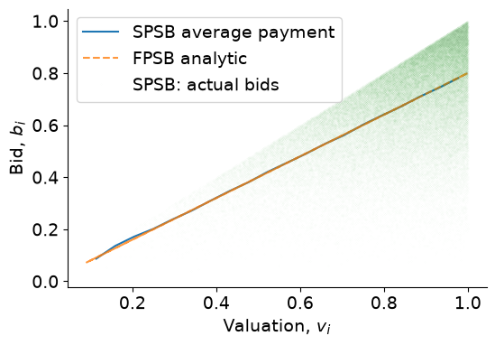
Let’s now plot the winning bids \(b_{(n)}\) (i.e. the payment) against valuations, \(v_{(n)}\) for both FPSB and SPSB.
Note that
FPSB: There is a unique bid corresponding to each valuation
SPSB: Because it equals the valuation of a second-highest bidder, what a winner pays varies even holding fixed the winner’s valuation. So here there is a frequency distribution of payments for each valuation.
# We intend to compute average payments of different groups of bidders
binned = stats.binned_statistic(v[-1, :], v[-2, :], statistic='mean', bins=20)
xx = binned.bin_edges
xx = [(xx[ii]+xx[ii+1])/2 for ii in range(len(xx)-1)]
yy = binned.statistic

fig, ax = plt.subplots(figsize=(6, 4))

ax.plot(xx, yy, label='SPSB average payment')
ax.plot(v[-1, :], b[-1, :], '--', alpha=0.8, label='FPSB analytic')
ax.plot(v[-1, :], v[-2, :], 'o', alpha=0.05,
                markersize=0.1, label='SPSB: actual bids')

ax.legend(loc='best')
ax.set_xlabel('Valuation, $v_i$')
ax.set_ylabel('Bid, $b_i$')
sns.despine()
140.9. Revenue equivalence theorem#
We now compare FPSB and a SPSB auctions from the point of view of the revenues that a seller can expect to acquire.
Expected Revenue FPSB:
The winner with valuation \(y\) pays \(\frac{n-1}{n} y\), where n is the number of bidders.
Above we computed that the CDF is \(F_{n}(y) = y^{n}\) and the PDF is \(f_{n} = ny^{n-1}\).
Consequently, expected revenue is
Expected Revenue SPSB:
The expected revenue equals n \(\times\) expected payment of a bidder.
Computing this we get
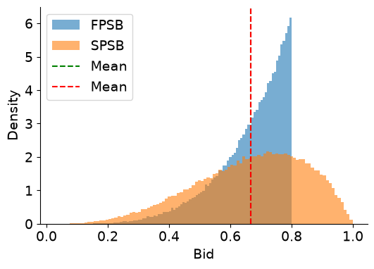
Thus, while probability distributions of winning bids typically differ across the two types of auction, we deduce that expected payments are identical in FPSB and SPSB.
fig, ax = plt.subplots(figsize=(6, 4))

for payment, label in zip([winner_pays_fpsb, winner_pays_spsb], ['FPSB', 'SPSB']):
    print('The average payment of %s: %.4f. Std.: %.4f. Median: %.4f' % (
        label, payment.mean(), payment.std(), np.median(payment)))
    ax.hist(payment, density=True, alpha=0.6, label=label, bins=100)

ax.axvline(winner_pays_fpsb.mean(), ls='--', c='g', label='Mean')
ax.axvline(winner_pays_spsb.mean(), ls='--', c='r', label='Mean')

ax.legend(loc='best')
ax.set_xlabel('Bid')
ax.set_ylabel('Density')
sns.despine()
The average payment of FPSB: 0.6670. Std.: 0.1122. Median: 0.6959
The average payment of SPSB: 0.6660. Std.: 0.1782. Median: 0.6850
Auction: Sealed-Bid |
First-Price |
Second-Price |
|---|---|---|
Winner |
Agent with highest bid |
Agent with highest bid |
Winner pays |
Winner’s bid |
Second-highest bid |
Loser pays |
0 |
0 |
Dominant strategy |
No dominant strategy |
Bidding truthfully is dominant strategy |
Bayesian Nash equilibrium |
Bidder \(i\) bids \(\frac{n-1}{n}v_{i}\) |
Bidder \(i\) truthfully bids \(v_{i}\) |
Auctioneer’s revenue |
\(\frac {n-1}{n+1}\) |
\(\frac {n-1}{n+1}\) |
Detour: Computing a Bayesian Nash Equibrium for FPSB
The revenue equivalence theorem lets us find an optimal bidding strategy for a FPSB auction from outcomes of a SPSB auction.
Let \(b(v_{i})\) be the optimal bid in a FPSB auction.
The revenue equivalence theorem tells us that a bidder agent with value \(v_{i}\) on average receives the same payment in the two types of auction.
Consequently,
It follows that an optimal bidding strategy in a FPSB auction is \(b(v_{i}) = \mathbb{E}_{y_{i}}[y_{i} | y_{i} < v_{i}]\).
140.10. Calculation of bid price in FPSB#
In equations (140.1) and (140.2), we displayed formulas for optimal bids in a symmetric Bayesian Nash equilibrium of a FPSB auction.
where
\(v_{i} = \) value of bidder \(i\)
\(y_{i} = \): maximum value of all bidders except \(i\), i.e., \(y_{i} = \max_{j \neq i} v_{j}\)
Above, we computed an optimal bid price in a FPSB auction analytically for a case in which private values are uniformly distributed.
For most probability distributions of private values, analytical solutions aren’t easy to compute.
Instead, we can compute bid prices in FPSB auctions numerically as functions of the distribution of private values.
def evaluate_largest(v_hat, array, order=1):
    """
    A method to estimate the largest (or certain-order largest) value of the other biders,
    conditional on player 1 wins the auction.

    We estimate E[y | y < v_hat], where y is the highest valuation among the
    other bidders.  We do this by taking bidder 1 as the reference bidder
    (valuations are IID, so the choice does not matter), discarding her row,
    and averaging the highest remaining valuation over those auctions in which
    every other bidder's valuation falls below v_hat.

    Parameters:
    ----------
    v_hat : float, the valuation of the reference bidder.

    array: 2 dimensional array of bidders' values in shape of (N,R),
           where N: number of players, R: number of auctions

    order: int. Which order statistic of the losing bidders to average.
                order=1 gives the highest losing valuation,
                order=2 the second highest, and so on.

    """
    N, R = array.shape

    # discard the reference bidder's row; condition on the rest losing
    array_residual = array[1:, :].copy()

    winning_auctions_mask = (array_residual < v_hat).all(axis=0)

    num_winning_auctions = np.sum(winning_auctions_mask)

    if num_winning_auctions == 0:
        return np.nan

    array_conditional = array_residual[:, winning_auctions_mask]

    array_conditional_sorted = np.sort(array_conditional, axis=0)

    order_largest_bids = array_conditional_sorted[-order, :]

    return np.mean(order_largest_bids)
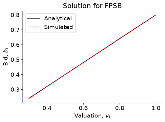
We can check the accuracy of our evaluate_largest method by comparing it with an analytical solution.
We find that the evaluate_largest method functions well
v_grid = np.linspace(0.3, 1, 8)
bid_analytical = b_star(v_grid, N)

# Redraw valuations
v = rng.uniform(0, 1, (N, R))
bid_simulated = [evaluate_largest(ii, v) for ii in v_grid]

fig, ax = plt.subplots(figsize=(6, 4))

ax.plot(v_grid, bid_analytical, '-', color='k', label='Analytical')
ax.plot(v_grid, bid_simulated, '--', color='r', label='Simulated')

ax.legend(loc='best')
ax.set_xlabel('Valuation, $v_i$')
ax.set_ylabel('Bid, $b_i$')
ax.set_title('Solution for FPSB')
sns.despine()
140.11. \(\chi^2\) Distribution#
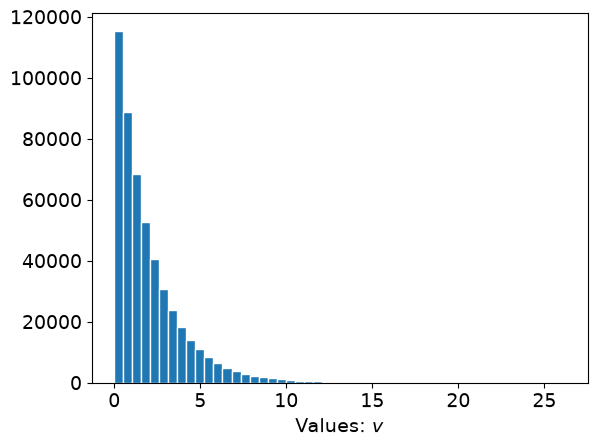
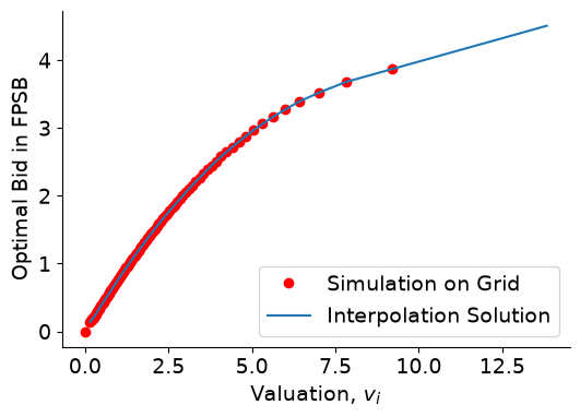
Let’s try an example in which the distribution of private values is a \(\chi^2\) distribution.
We’ll start by taking a look at a \(\chi^2\) distribution with the help of the following Python code:
rng = np.random.default_rng(1337)
v = rng.chisquare(df=2, size=(N * R,))

plt.hist(v, bins=50, edgecolor='w')
plt.xlabel('Values: $v$')
plt.show()
Now we’ll get Python to construct a bid price function
rng = np.random.default_rng(1337)
v = rng.chisquare(df=2, size=(N, R))

# we compute the quantile of v as our grid
pct_quantile = np.linspace(0, 100, 101)[1:-1]
v_grid = np.percentile(v.flatten(), q=pct_quantile)

# nan values are returned for some low quantiles due to lack of observations
EV = [evaluate_largest(ii, v) for ii in v_grid]
# we insert 0 into our grid and bid price function as a complement
EV = np.insert(EV, 0, 0)
v_grid = np.insert(v_grid, 0, 0)

b_star_num = interp.interp1d(v_grid, EV, fill_value="extrapolate")
We check our bid price function by computing and visualizing the result.
pct_quantile_fine = np.linspace(0, 100, 1001)[1:-1]
v_grid_fine = np.percentile(v.flatten(), q=pct_quantile_fine)

fig, ax = plt.subplots(figsize=(6, 4))

ax.plot(v_grid, EV, 'or', label='Simulation on Grid')
ax.plot(v_grid_fine, b_star_num(v_grid_fine),
                '-', label='Interpolation Solution')

ax.legend(loc='best')
ax.set_xlabel('Valuation, $v_i$')
ax.set_ylabel('Optimal Bid in FPSB')
sns.despine()
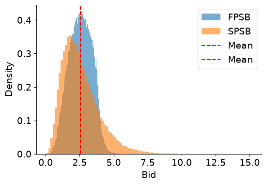
Now we can use Python to compute the probability distribution of the price paid by the winning bidder
b = b_star_num(v)

idx = np.argsort(v, axis=0)
# same as np.sort(v, axis=0), except now we retain the idx
v = np.take_along_axis(v, idx, axis=0)
b = np.take_along_axis(b, idx, axis=0)

# highest bid
winner_pays_fpsb = b[-1, :]
# 2nd-highest valuation
winner_pays_spsb = v[-2, :]
fig, ax = plt.subplots(figsize=(6, 4))

for payment, label in zip([winner_pays_fpsb, winner_pays_spsb],
                          ['FPSB', 'SPSB']):
    print('The average payment of %s: %.4f. Std.: %.4f. Median: %.4f' % (
        label, payment.mean(), payment.std(), np.median(payment)))
    ax.hist(payment, density=True, alpha=0.6, label=label, bins=100)

ax.axvline(winner_pays_fpsb.mean(), ls='--', c='g', label='Mean')
ax.axvline(winner_pays_spsb.mean(), ls='--', c='r', label='Mean')

ax.legend(loc='best')
ax.set_xlabel('Bid')
ax.set_ylabel('Density')
sns.despine()
The average payment of FPSB: 2.5672. Std.: 0.8373. Median: 2.5794
The average payment of SPSB: 2.5634. Std.: 1.3637. Median: 2.3075
140.12. Code summary#
We assemble the functions that we have used into a Python class
class bid_price_solution:

    def __init__(self, array):
        """
        A class that can plot the value distribution of bidders,
        compute the optimal bid price for bidders in FPSB
        and plot the distribution of winner's payment in both FPSB and SPSB

        Parameters:
        ----------

        array: 2 dimensional array of bidders' values in shape of (N, R),
               where N: number of players, R: number of auctions

        """
        self.value_mat = array.copy()

        return None

    def plot_value_distribution(self):
        plt.hist(self.value_mat.flatten(), bins=50, edgecolor='w')
        plt.xlabel('Values: $v$')
        plt.show()

        return None

    def evaluate_largest(self, v_hat, order=1):
        N, R = self.value_mat.shape

        # drop the first row because we assume first row is the winner's bid
        array_residual = self.value_mat[1:, :].copy()

        winning_auctions_mask = (array_residual < v_hat).all(axis=0)

        num_winning_auctions = np.sum(winning_auctions_mask)

        if num_winning_auctions == 0:
            return np.nan

        array_conditional = array_residual[:, winning_auctions_mask]
        array_conditional_sorted = np.sort(array_conditional, axis=0)
        order_largest_bids = array_conditional_sorted[-order, :]

        return np.mean(order_largest_bids)

    def compute_optimal_bid_FPSB(self, plot=True):
        # we compute the quantile of v as our grid
        pct_quantile = np.linspace(0, 100, 101)[1:-1]
        v_grid = np.percentile(self.value_mat.flatten(), q=pct_quantile)

        # nan values are returned for some low quantiles due to lack of observations
        EV = [self.evaluate_largest(ii) for ii in v_grid]

        # we insert 0 into our grid and bid price function as a complement
        EV = np.insert(EV, 0, 0)
        v_grid = np.insert(v_grid, 0, 0)

        self.b_star_num = interp.interp1d(v_grid, EV,
                                           fill_value="extrapolate")

        if not plot:
            return None

        pct_quantile_fine = np.linspace(0, 100, 1001)[1:-1]
        v_grid_fine = np.percentile(self.value_mat.flatten(),
                                    q=pct_quantile_fine)

        fig, ax = plt.subplots(figsize=(6, 4))

        ax.plot(v_grid, EV, 'or', label='Simulation on Grid')
        ax.plot(v_grid_fine, self.b_star_num(v_grid_fine),
                            '-', label='Interpolation Solution')

        ax.legend(loc='best')
        ax.set_xlabel('Valuation, $v_i$')
        ax.set_ylabel('Optimal Bid in FPSB')
        sns.despine()

        return None

    def plot_winner_payment_distribution(self):
        if not hasattr(self, 'b_star_num'):     # bids have not been computed yet
            self.compute_optimal_bid_FPSB(plot=False)

        self.b = self.b_star_num(self.value_mat)

        idx = np.argsort(self.value_mat, axis=0)
        # same as np.sort(v, axis=0), except now we retain the idx
        self.v = np.take_along_axis(self.value_mat, idx, axis=0)
        self.b = np.take_along_axis(self.b, idx, axis=0)

        # highest bid
        winner_pays_fpsb = self.b[-1, :]
        # 2nd-highest valuation
        winner_pays_spsb = self.v[-2, :]

        fig, ax = plt.subplots(figsize=(6, 4))

        for payment, label in zip([winner_pays_fpsb, winner_pays_spsb],
                                   ['FPSB', 'SPSB']):
            print('The average payment of %s: %.4f. Std.: %.4f. Median: %.4f' %
                  (label, payment.mean(), payment.std(), np.median(payment)))
            ax.hist(payment, density=True, alpha=0.6, label=label, bins=100)

        ax.axvline(winner_pays_fpsb.mean(), ls='--', c='g', label='Mean')
        ax.axvline(winner_pays_spsb.mean(), ls='--', c='r', label='Mean')

        ax.legend(loc='best')
        ax.set_xlabel('Bid')
        ax.set_ylabel('Density')
        sns.despine()

        return None
rng = np.random.default_rng(1337)
v = rng.chisquare(df=2, size=(N, R))

chi_squ_case = bid_price_solution(v)
chi_squ_case.plot_value_distribution()
chi_squ_case.compute_optimal_bid_FPSB()
chi_squ_case.plot_winner_payment_distribution()
The average payment of FPSB: 2.5672. Std.: 0.8373. Median: 2.5794
The average payment of SPSB: 2.5634. Std.: 1.3637. Median: 2.3075
140.13. Exercises#
Exercise 140.1
Verify the revenue equivalence theorem by simulation.
For \(n = 2, 3, 5, 10\) bidders with valuations drawn independently from \(U(0,1)\), simulate many auctions and compute
the average payment of the winner in a FPSB auction, in which each bidder bids \(\frac{n-1}{n} v_i\)
the average payment of the winner in a SPSB auction, in which each bidder bids \(v_i\)
Compare both with the theoretical expected revenue \(\frac{n-1}{n+1}\), and comment on how the seller’s revenue changes with the number of bidders.
Solution
R_ex = 200_000
rng_ex = np.random.default_rng(1234)

print(f"{'n':>4}{'FPSB':>12}{'SPSB':>12}{'(n-1)/(n+1)':>14}")
for n in (2, 3, 5, 10):
    v_ex = np.sort(rng_ex.uniform(0, 1, (n, R_ex)), axis=0)
    fpsb = (n - 1)/n * v_ex[-1, :]      # winner's own bid
    spsb = v_ex[-2, :]                  # second highest valuation
    print(f"{n:>4}{fpsb.mean():>12.4f}{spsb.mean():>12.4f}{(n-1)/(n+1):>14.4f}")
   n        FPSB        SPSB   (n-1)/(n+1)
   2      0.3335      0.3340        0.3333
   3      0.5000      0.5000        0.5000
   5      0.6671      0.6676        0.6667
  10      0.8185      0.8185        0.8182
The two auctions raise the same expected revenue, and both converge to the highest possible valuation as \(n\) grows.
With more bidders, competition pushes the winning payment toward the top of the support of valuations.
Notice that the two auctions raise the same revenue on average even though the distributions of the winner’s payment differ: in a FPSB auction the payment is a deterministic function of the winner’s valuation, while in a SPSB auction it is the second-highest valuation, which is random given the winner’s valuation.
Exercise 140.2
Equation (140.1) says that an optimal bid in a FPSB auction is \(\mathbb{E}[y_i \mid y_i < v_i]\).
Show that this can be written
\[ b(v) = v - \frac{\int_0^{v} F(x)^{n-1} dx}{F(v)^{n-1}} \]where \(F\) is the distribution function of a valuation.
Verify that this reduces to \(\frac{n-1}{n}v\) when \(F\) is uniform on \([0,1]\).
Evaluate the formula for a \(\chi^2(2)\) distribution of valuations and compare it with the simulation-based bid function computed in the lecture.
Solution
The distribution function of \(y_i = \max_{j \neq i} v_j\) is \(\tilde F_{n-1}(y) = F(y)^{n-1}\).
Hence
Integrating by parts,
which gives the formula.
For \(F(x) = x\) on \([0,1]\) we get \(b(v) = v - \frac{v^n/n}{v^{n-1}} = \frac{n-1}{n} v\).
The formula has a nice reading: a bidder shades her bid below her valuation by an amount that shrinks as the number of competitors grows.
from scipy.integrate import quad

def b_closed_form(v, F, n):
    "Optimal FPSB bid for a bidder with valuation v when rivals' values ~ F."
    shading = quad(lambda x: F(x)**(n - 1), 0, v)[0] / F(v)**(n - 1)
    return v - shading

# check against the analytical solution for the uniform case
print("uniform check")
for v0 in (0.3, 0.6, 0.9):
    print(f"  v = {v0}:  closed form {b_closed_form(v0, lambda x: x, N):.4f}, "
          f"analytical {b_star(v0, N):.4f}")
uniform check
  v = 0.3:  closed form 0.2400, analytical 0.2400
  v = 0.6:  closed form 0.4800, analytical 0.4800
  v = 0.9:  closed form 0.7200, analytical 0.7200
# now the chi-squared case studied in the lecture
F_chi2 = stats.chi2(df=2).cdf
v_test = np.percentile(v.flatten(), [10, 30, 50, 70, 90])

print(f"{'v':>8}{'closed form':>14}{'simulated':>12}")
for v0 in v_test:
    print(f"{v0:>8.3f}{b_closed_form(v0, F_chi2, N):>14.4f}"
          f"{float(b_star_num(v0)):>12.4f}")
       v   closed form   simulated
   0.210        0.1663      0.1825
   0.711        0.5513      0.5544
   1.383        1.0370      1.0433
   2.397        1.6965      1.6984
   4.607        2.8055      2.7974
The closed form and the simulation agree closely, which is a useful check on both.
Exercise 140.3
This exercise asks you to see why truthful bidding is a weakly dominant strategy in a SPSB auction but not in a FPSB auction.
Fix \(n = 5\) and consider a bidder whose valuation is \(v = 0.75\), facing rivals whose valuations are \(U(0,1)\).
In a SPSB auction the rivals bid truthfully. Compute this bidder’s expected surplus as a function of her own bid \(b\) and plot it.
In a FPSB auction the rivals bid \(\frac{n-1}{n}v_j\). Compute and plot her expected surplus as a function of \(b\).
Where does each curve peak? What surplus does she earn in the FPSB auction if she bids her valuation?
Solution
In the SPSB auction she wins when \(y < b\) and then pays \(y\), so her expected surplus is
Differentiating with respect to \(b\) gives \((v-b)(n-1)b^{n-2}\), which is positive for \(b < v\) and negative for \(b > v\), so \(b = v\) is optimal.
In the FPSB auction she wins when every rival’s bid falls below \(b\), which happens with probability \(\left(\frac{nb}{n-1}\right)^{n-1}\), and then she pays \(b\).
n_ex, v_own = 5, 0.75
bids = np.linspace(0, 1, 401)

spsb_surplus = [quad(lambda y: (v_own - y)*(n_ex - 1)*y**(n_ex - 2),
                     0, min(bb, 1))[0] for bb in bids]
fpsb_surplus = [(v_own - bb)*min(1, n_ex*bb/(n_ex - 1))**(n_ex - 1)
                for bb in bids]

fig, ax = plt.subplots(figsize=(6, 4))
ax.plot(bids, spsb_surplus, label='SPSB')
ax.plot(bids, fpsb_surplus, label='FPSB')
ax.axvline(v_own, ls='--', c='k', lw=1, label='own valuation')
ax.axvline((n_ex - 1)/n_ex*v_own, ls=':', c='r', lw=1, label='FPSB optimal bid')
ax.set_xlabel('own bid $b$')
ax.set_ylabel('expected surplus')
ax.legend()
plt.show()

print(f"SPSB surplus is maximized at b = {bids[int(np.argmax(spsb_surplus))]:.3f}")
print(f"FPSB surplus is maximized at b = {bids[int(np.argmax(fpsb_surplus))]:.3f}"
      f"  (theory: {(n_ex - 1)/n_ex*v_own:.3f})")
print(f"FPSB surplus from bidding one's valuation: {(v_own - v_own):.3f}")
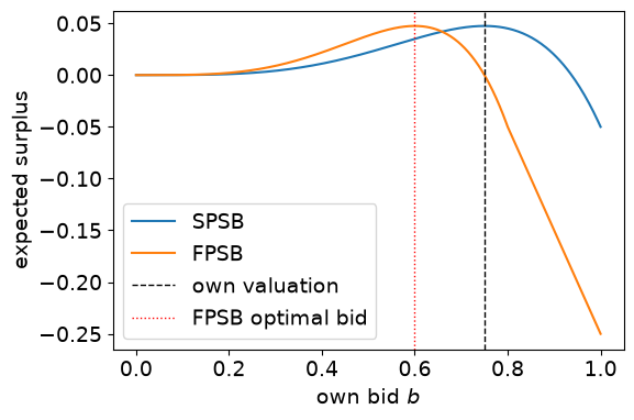
SPSB surplus is maximized at b = 0.750
FPSB surplus is maximized at b = 0.600  (theory: 0.600)
FPSB surplus from bidding one's valuation: 0.000
The SPSB curve peaks exactly at the bidder’s valuation.
The FPSB curve peaks strictly below it, and bidding one’s valuation in a FPSB auction earns a surplus of exactly zero: the bidder wins more often, but pays her full valuation whenever she does.
Exercise 140.4
The revenue equivalence theorem requires bidders to be risk neutral.
Suppose instead that each bidder has utility \(u(x) = x^\rho\) with \(0 < \rho \leq 1\), so that \(\rho < 1\) means risk aversion, and that valuations are \(U(0,1)\).
One can show that the symmetric equilibrium bid in a FPSB auction becomes
Verify this numerically: for \(n = 5\) and a bidder with \(v = 0.8\), compute expected utility as a function of her own bid when rivals use this rule, and check where it is maximized.
Compute the seller’s expected revenue in FPSB and SPSB for \(\rho = 1, 0.6, 0.3\).
Explain the intuition.
Solution
def expected_utility(b, v_own, n, ρ):
    "Expected utility of bidding b when rivals bid (n-1)v/(n-1+ρ)."
    win_prob = np.minimum(1, b*(n - 1 + ρ)/(n - 1))**(n - 1)
    return win_prob * np.maximum(v_own - b, 0)**ρ

n_ex, v_own = 5, 0.8
grid = np.linspace(0.001, v_own, 2001)

print(f"{'ρ':>6}{'theory b*':>12}{'numerical':>12}")
for ρ in (1.0, 0.5, 0.2):
    theory = (n_ex - 1)*v_own/(n_ex - 1 + ρ)
    numerical = grid[int(np.argmax(expected_utility(grid, v_own, n_ex, ρ)))]
    print(f"{ρ:>6}{theory:>12.4f}{numerical:>12.4f}")
     ρ   theory b*   numerical
   1.0      0.6400      0.6398
   0.5      0.7111      0.7109
   0.2      0.7619      0.7620
rng_ra = np.random.default_rng(42)
v_ra = np.sort(rng_ra.uniform(0, 1, (n_ex, 200_000)), axis=0)

print(f"{'ρ':>6}{'FPSB revenue':>15}{'SPSB revenue':>15}")
for ρ in (1.0, 0.6, 0.3):
    fpsb = ((n_ex - 1)/(n_ex - 1 + ρ)) * v_ra[-1, :]
    print(f"{ρ:>6}{fpsb.mean():>15.4f}{v_ra[-2, :].mean():>15.4f}")
     ρ   FPSB revenue   SPSB revenue

   1.0         0.6666         0.6668
   0.6         0.7245         0.6668
   0.3         0.7751         0.6668
With risk neutrality (\(\rho = 1\)) the two auctions raise the same revenue, as the theorem says.
With risk aversion (\(\rho < 1\)) the FPSB auction raises more.
The intuition is that in a FPSB auction, shading one’s bid is a gamble: it raises the surplus conditional on winning but lowers the probability of winning.
A risk-averse bidder dislikes that gamble and so shades less, which transfers revenue to the seller.
In a SPSB auction the winner’s payment does not depend on her own bid, so risk aversion changes nothing: bidding one’s valuation remains weakly dominant, and the seller’s revenue is unaffected.
140.14. Further reading#
The second-price sealed-bid auction was proposed by Vickrey [1961].
For textbook treatments of the material in this lecture, see Krishna [2009] and Milgrom [2004].
Klemperer [1999] surveys the literature.
The revenue equivalence theorem in the general form sketched above is due to Myerson [1981] and Riley and Samuelson [1981].
Both auctions studied here are naturally described in terms of order statistics of bidders’ valuations, a subject treated at length by David and Nagaraja [2003].